Making an antigenic map from titer data
Source:vignettes/making-a-map-from-scratch.Rmd
making-a-map-from-scratch.RmdIn this vignette we’re going to go through the process of making an antigenic map using Racmacs and viewing and saving the resulting map and images and interactive plots of the map.
The steps will be:
- Reading in the titer data
- Creating the acmap object
- Running a set of optimizations to try and find the best map to represent the data
- Viewing the map
- Saving the map
Reading in the titer data
First of all we need to read in the titer data from a file, exactly how you do this depends on the format of your data but ultimately you need to end up with a matrix or dataframe of titers where rows represent antigens and columns represent sera.
If your titer data is in a simple format where you just have a single
header for serum names and a single first column of antigen names you
can try using the function read.titerTable(), as in the
example below.
For this example we will be reading the titer data from the first antigenic map of H3N2 antigenic evolution, published in 2004 and included with the Racmacs package.
# Load the Racmacs package
library(Racmacs)

# Set an option for the number of computer cores to run in parallel when optimizing maps
# The default when running on CRAN is to use 2
options(RacOptimizer.num_cores = 1)
# However you can also set the number of cores to the maximum number like this
# options(RacOptimizer.num_cores = parallel::detectCores())

# Read in the titer table
path_to_titer_file <- system.file("extdata/h3map2004_hitable.csv", package = "Racmacs")
titer_table        <- read.titerTable(path_to_titer_file)
The resulting titer table is a matrix of titers with column and row names:
print(titer_table[1:5,1:7])
#>             HK/1/68 HK/107/71 BI/21793/72 EN/42/72 PC/1/73 BI/5930/74 SL/840/74
#> BI/15793/68 "354"   "*"       "*"         "501"    "109"   "*"        "*"
#> BI/16190/68 "640"   "*"       "640"       "320"    "80"    "320"      "40"
#> BI/16398/68 "1163"  "*"       "*"         "1163"   "291"   "*"        "73"
#> HK/1/68     "1280"  "1280"    "*"         "2560"   "53"    "*"        "<10"
#> BI/808/69   "320"   "*"       "*"         "640"    "120"   "*"        "80"
Creating the acmap object
Now we have the titers in the correct format we can use it create an
antigenic map object or “acmap” object. For this we use the constructor
function acmap(), akin to how data.frame() is
used to make a data frame object or matrix() for a
matrix.
# Create the acmap object, specifying the titer table
map <- acmap(
  titer_table = titer_table
)
The resulting object, that we’ve given the name map in
this case, only has properties associated with the table. If the table
had column names and row names, serum and antigen names are inferred
from these. Alternatively, you can set these explicitly when creating
the map with the ag_names and sr_names
arguments.
Running optimizations
Although we now have the acmap object there is no “map” yet as such,
since we need to invoke the optimiser function to try and determine the
antigenic map that best represents the patterns of reactivity seen in
the titer table. To do this we call the function
optimizeMap() on the acmap object we’ve made, specifying
the number of optimization runs and other parameters like the minimum
column basis and number of dimensions.
In this case we’re going to try and find the best 2-dimensional solution for the map data, using 500 optimization runs.
# Perform some optimization runs on the map object to try and determine a best map
map <- optimizeMap(
  map                     = map,
  number_of_dimensions    = 2,
  number_of_optimizations = 500,
  minimum_column_basis    = "none"
)
#> a
#> Took 50 secs
#> Warning in optimizeMap(map = map, number_of_dimensions = 2,
#> number_of_optimizations = 500, : There is some variation (9.57 AU for one
#> point) in the top runs, this may be an indication that more optimization runs
#> could help achieve a better optimum. If this still fails to help see
#> ?unstableMaps for further possible causes.
By default the resulting map optimizations are sorted by their stress, so that the optimization that resulted in the lowest map stress (i.e. usually thought of as the best solution), will be first and will be the default optimization run selected and therefore will be the one used when querying anything like antigen and serum coordinates, map stress etc. unless otherwise specified.
Viewing the map
The lowest stress optimization run will also be the one used by
default when viewing the map. To view the map, you can either do a
simple plot of the map using the plot() function
plot(map)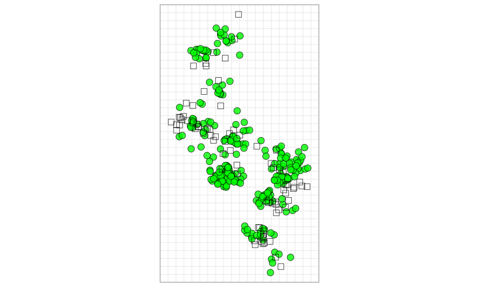
or you can view the map interactively using the view()
function
view(map)Using make.acmap()
Note that there is also a small utility function provided to allow
you to create the acmap object and run optimizations on it all in one
step. In the example below we use it to create a 3d version of the
antigenic map and then use view() map to view the result
(plot() will not work with 3 dimensional maps).
# Make the acmap object and run optimizations
map3d <- make.acmap(
  titer_table             = titer_table,
  number_of_dimensions    = 3,
  number_of_optimizations = 500,
  minimum_column_basis    = "none"
)
#> a
#> Warning: The following SERA have do not have enough titrations to position in 3 dimensions. Coordinates were still optimized but positions will be unreliable
#>
#> 'HK/107/71'
#> Took 1.64 mins
#> Warning in optimizeMap(map = map, number_of_dimensions = number_of_dimensions,
#> : There is some variation (5.14 AU for one point) in the top runs, this may be
#> an indication that more optimization runs could help achieve a better optimum.
#> If this still fails to help see ?unstableMaps for further possible causes.

# View the result
view(map3d)